前言 比特币(Bitcoin)是2008年一个自称名为中本聪(Satoshi Nakamoto)的人在互联网上发布的一套加密交易协议1
ARIMA(Autoregressive Integrated Moving Average)模型是金融时间序列分析中常用的工具2
本文将详细介绍如何使用Python中相关的程序包实现基于ARIMA模型的比特币收益率预测。
数据分析 首先从yahoo finance上下载bitcoin日度行情数据。
1
2
3
4
5
6
7
8
9
10
11
from datetime import datetimefrom pandas_datareader import data as pdrimport yfinance as yfyf.pdr_override() start_date = datetime(2015 ,1 ,1 ) end_date = datetime(2023 ,6 ,30 ) df_btc_price = pdr.get_data_yahoo('BTC-USD' , start=start_date, end=end_date, interval='1d' ) df_btc_price.index = df_btc_price.index.astype('datetime64[ns]' ) df_btc_price.head()
1
2
3
4
import matplotlib.pyplot as pltplt.plot(df_btc_price['Close' ]) plt.show()
从图中可以推测价格数据不平稳,下面做一下adf检验平稳性。
1
2
3
from statsmodels.tsa.stattools import adfullerprint ('price time series adfuller p-value:' , adfuller(df_btc_price['Close' ])[1 ])
1 price time series adfuller p-value: 0.5158389287588319
P值非常大,证明价格数据不平稳。
1
2
returns = df_btc_price['Close' ].pct_change().dropna() plt.plot(returns)
从图上看收益率序列有稳定均值,且围绕均值上下波动,波动幅度也较为稳定。下面进行adf检验。
1 print ('return timeseries adfuller p-value:' , adfuller(returns)[1 ])
1 return timeseries adfuller p-value: 0.0
P值验证收益率序列是平稳的。关于adf检验的原理可以参考ADF检验 。
下面将数据拆分为训练集和测试集,训练集主要用于模型参数优化,测试集进行样本外模型绩效评估。
1
2
3
4
5
import mathtraining_data_len = math.ceil(len (returns) * .8 ) returns_train = returns.loc[:training_data_len] returns_test = returns.loc[training_data_len:]
ARIMA 模型 下面准备使用ARIMA模型建模,ARIMA模型中一共有三个参数, p, d, q:
p: AR 部分阶数
d: I 部分差分次数
q: MA 部分阶数
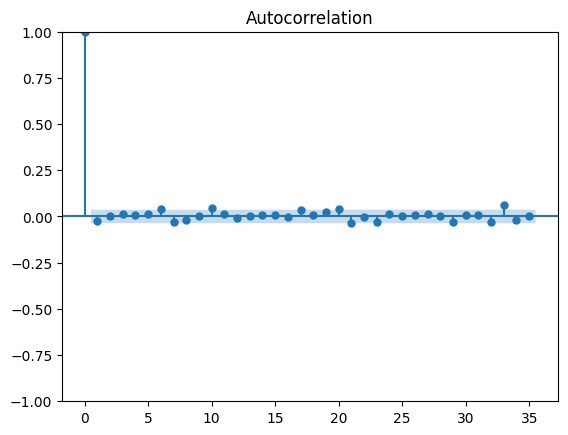
首先手动选取一个模型进行分析,根据Tsay(2009),可以使用acf来选取MA部分参数q。
1
2
3
4
from statsmodels.graphics.tsaplots import plot_acfplot_acf(returns_train) plt.show()
从图中可以看出lag为6,10时相关性较大,手动选取(0,0,6)为作为ARIMA参数测试。
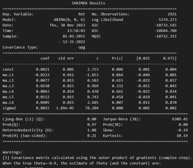
1
2
3
4
5
6
7
8
9
10
11
from statsmodels.tsa.arima.model import ARIMAmod = ARIMA(returns_train, order=(0 , 0 , 6 )) res = mod.fit() print (res.summary())print ("When the true theta=-0.9, the estimate of theta (and the constant) are:" )print (res.params)
6项系数标准错误在0.012-015之间,LB 检验值为0.00,p-LB为0.97,拟合结果可以接受。3 4
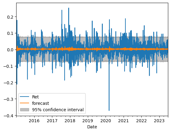
1
2
3
4
5
6
7
8
9
10
import matplotlib.pyplot as pltimport pandas as pdimport statsmodels.api as smfrom statsmodels.graphics.tsaplots import plot_predictfrom statsmodels.tsa.arima.model import ARIMAfig, ax = plt.subplots() ax = returns.plot(ax=ax) plot_predict(res, ax=ax) plt.show()
样本内预测值与实际值的统计情况如上,其中阴影部分为95%置信区间。
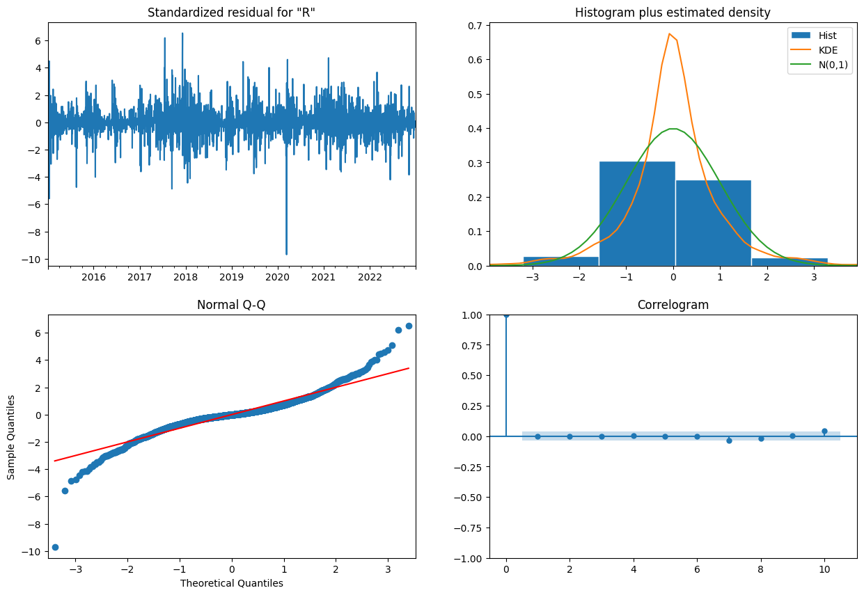
预测残差如下统计信息。
1
2
res.plot_diagnostics(figsize = (15 , 10 )) plt.show()
预测RMSE (Root mean squared error)
1
2
3
4
5
from sklearn.metrics import mean_squared_errorfrom math import sqrtrms = sqrt(mean_squared_error(returns_train, res.predict())) print ('Training RMSE: %.3f' % rms)
Grid-Search 优化参数 为了选取最优模型,使用grid search方法遍历组合进行拟合,并选取AIC最小的模型参数。
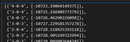
1
2
3
4
5
6
7
8
9
10
11
12
13
14
15
16
17
18
19
20
21
22
23
24
25
26
27
28
29
30
31
32
33
34
def iterative_ARIMA_fit (series ): """ Iterates within the allowed values of the p and q parameters Returns a dictionary with the successful fits. Keys correspond to models. """ ARrange = range (0 , 5 ) MArange = range (0 , 5 ) Diffrange = [0 ] ARIMA_fit_results = {} for AR in ARrange : for MA in MArange : for Diff in Diffrange: params = (AR,Diff,MA) series.freq ='D' print (params) model = ARIMA(series, order = params) try : results_ARIMA = model.fit() aic = results_ARIMA.aic ARIMA_fit_results['%d-%d-%d' % (AR,Diff,MA)]=[aic] except : continue return ARIMA_fit_results opt_result = iterative_ARIMA_fit(returns_train) sorted (opt_result.items(), key=lambda item: item[1 ], reverse=True )
选取参数 4, 0, 4进行样本外检验
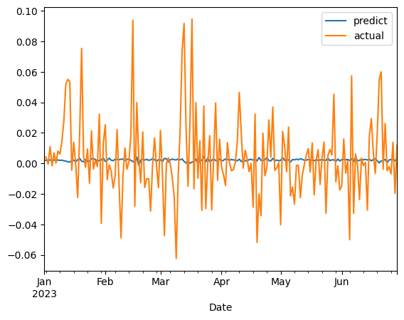
1
2
3
4
5
6
7
8
9
10
11
12
13
14
15
16
17
18
19
20
21
22
23
24
25
26
27
28
29
def rolling_predict (returns_train, returns_test, order_params ): """ rolling forcasting arima model """ history = returns_train.to_list() test = returns_test.to_list() test_index = returns_test.index predictions = [] actuals = [] for t in range (len (test)): model = ARIMA(history, order=order_params) res = model.fit() output = res.forecast() yhat = output[0 ] predictions.append(yhat) obs = test[t] actuals.append(obs) history.append(obs) df_predict = pd.DataFrame(index=test_index, columns=['predict' , 'actual' ]) df_predict['predict' ] = predictions df_predict['actual' ] = actuals return df_predict pred_rolling = rolling_predict(returns_train, returns_test, (4 ,0 ,4 )) pred_rolling.dropna().plot()
1 2 3 4 5 6 from sklearn.metrics import mean_squared_errorfrom math import sqrtrmse = sqrt(mean_squared_error(pred_rolling['actual' ], pred_rolling['predict' ])) print ('test RMSE: ' , rmse)
1 test RMSE: 0.025680854707355105
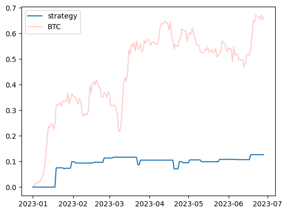
用一个简单的策略进行验证,在下一日预测收益率大于0.003时做多,否则平仓。
1
2
3
4
5
6
7
8
9
10
11
12
13
14
15
16
17
18
19
def test_strategy (df_returns, open_long_threshold=0.005 ): """ test strategy, if predict > threshold, open long, close otherwise. """ df_strategy = pd.DataFrame(index=df_returns.index) df_strategy['weight' ] = df_returns['predict' ].apply(lambda x: 1.0 if x > open_long_threshold else 0.0 ) df_strategy['act_return' ] = df_returns['actual' ].shift(-1 ) df_strategy['ret_contrib' ] = df_strategy['weight' ] * df_strategy['act_return' ] return df_strategy def plot_strategy (df_strategy ): fig, ax = plt.subplots() ax.plot(df_strategy['ret_contrib' ].cumsum(), label='strategy' ) ax.plot(df_strategy['act_return' ].cumsum(), color='red' , alpha=0.2 , label='BTC' ) plt.legend() plt.show() df_strategy_result = test_strategy(pred_rolling, open_long_threshold=0.003 ) plot_strategy(df_strategy_result)
从回测可以看出,本策略可以今年上半年收益约10%,躲过了大部分回撤。
总结 在本文中大虾演示了从数据分析到ARIMA建模,再到模型参数优化和模拟策略回测。ARIMA模型在比特币收益率预测上表现不错,但是由于比特币价格波动较大,预测收益率的误差也较大,需要进一步优化模型或者使用其他模型进行预测。
参考资料